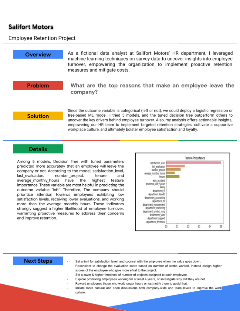
Summary: The project aims to address the problem of high turnover rate among employees for Salifort Motors. By analyzing their survey data and designing predictive models, I, as a fictional data professional, identified key factors driving turnover and proposed solutions to enhance retention and save costs.
About: This project is a Capstone project of Google Advanced Data Analytics specialization. The Specialization consists of 7 courses, and this capstone project is the very last project to get the certification from Google. So, I have been excited about this project. It allowed me to apply skills gathered from the whole program, including Python, EDA, Data visualizations, statistics, Machine Learning Modeling, PACE workflow, etc. In addition, I was also responsible for solving a particular business problem in an imaginary organizational setup such as setting up the team’s workflow, creating a project proposal, interacting with a variety of internal and external stakeholders, and sharing insights & final recommendations through an executive summary.
About the Company
Salifort Motors is a (fictional) French-based alternative energy vehicle manufacturer. Its global workforce of over 100,000 employees research, design, construct, validate, and distribute electric, solar, algae, and hydrogen-based vehicles. Salifort’s end-to-end vertical integration model has made it a global leader at the intersection of alternative energy and automobiles.
Business Case Scenario
“As a data specialist working for Salifort Motors, I have received the results of a recent employee survey. The senior leadership team has tasked me with analyzing the data to come up with ideas for how to increase employee retention. To help with this, they would like me to design a model that predicts whether an employee will leave the company based on their department, number of projects, average monthly hours, and any other data points you deem helpful.”
Stakeholders: Senior Leadership team, and the head of HR.
Goal: Identify the factors that cause high employee turnover, and predict if an employee will leave the company or not.
Resources: The Survey dataset, Python Jupyter Notebook, and any additional input from stakeholders.
Data Source: Link
Solution: With PACE workflow, I completed the project in these 4 steps
- Initial Exploratory Data Analysis (EDA)
- Analysis of variables
- Build ML models
- Summerize results & provide recommendations.
Data Dictionary
This project uses a dataset called HR_capstone_dataset.csv. It represents 10 columns of self-reported information from employees of a multinational vehicle manufacturing corporation.
The dataset contains:
14,999 rows – each row is a different employee’s self-reported information
10 columns
Column name
satisfaction_level
last_evaluation
number_project
average_monthly_hours
time_spend_company
work_accident
left
promotion_last_5years
department
salary
Description
The employee’s self-reported satisfaction level [0-1]
Score of employee’s last performance review[0-1]
Number of projects employee contributes to
Average number of hours employee worked per month
How long the employee has been with the company
Whether or not the employee experienced an accident at work
Whether or not the employee left the company
Whether or not the employee was promoted in the last 5 years.
The employee’s department
The employee’s salary [low, medium, high]
Type
int64
int64
int64
int64
int64
int64
int64 int64
str
str
I completed this Project Workflow using PACE model to keep myself organised!
Milestones
Tasks
PACE stages
1
Project Workflow is outlined
Complete Strategy & Proposal document
Data is loaded into the Jupyter Notebook.
*Deliverables: Documents (Project workflow, Project proposal, Project strategy)
Plan
2
Basic structure & descriptive stats are checked
Data is scrubbed & formatted, Key features are selected
Outliers are detected & Handled
Dataset is ready for modeling.
*Deliverables: Clean Dataset with relevant features
Analyze
3
Modeling and machine learning decisions are finalized.
Model is constructed
Machine learning techniques are tested and retested for accuracy
*Deliverables: Machine Learning Model
Construct
4
Results are finalized
Findings are shared with stakeholders
Feedback is incorporated
*Deliverables: Visualizations, Executive Summary, results.
Execute
Milestones | Tasks | PACE stages |
1 |
*Deliverables: Documents (Project workflow, Project proposal, Project strategy) | Plan |
2 |
*Deliverables: Clean Dataset with relevant features | Analyze |
3 |
*Deliverables: Machine Learning Model | Construct |
4 |
*Deliverables: Visualizations, Executive Summary, results. | Execute |

Step 1: Exploratory Data Analysis (EDA)
Before constructing a predictive model, it is important to know features, their relationships, distributions, etc. EDA is an approach to analyzing datasets to summarizing their main characteristics, often with visual methods. The goal of EDA is to gain insights from the data, understand its underlying structure and distributions, identify patterns, detect anomalies, and formulate hypotheses for further investigation.
In this step, I performed 4 tasks in total (Load dataset, data exploration, data cleaning, and analyze data) with subtasks included and observed interesting information which I also shared here –
1. Loaded dataset with using read_csv() method.
3. Data Cleaning
- Renamed misspelled & incorrect columns as per the standardized snake_case rule, and made as concise as needed, such as (tenure: time_spend_company)
- Checked missing & duplicate values by isna() and duplicated() methods; found 3008 duplicate values, dropped them with drop_duplicates().
- Checked outliers in each variable using boxplot, only tenure showed some influential values.
2. Data Exploration
- Gathered basic information, such as the number of records, and datatypes, using info() method.
- Gathered descriptive statistics such as counts, mean, median, max etc. values of the data using describe().
4. Outliers handling
- Implemented 3 methods learnt from the Google Specialization for outlier detection and handling: using z-score, standard deviation and interquartile range.
- Among these 3, I detected more values (824) as outliers by calculating percentile and interquartile range. So, I designed an imputer function to cut down these outliers and set them under the upper & lower thresholds.

Step 2: Analyze relationship between variables (EDA)
In the Analyze stage of the project, I conducted a comprehensive examination of our survey data to unearth insights into employee turnover. 📊
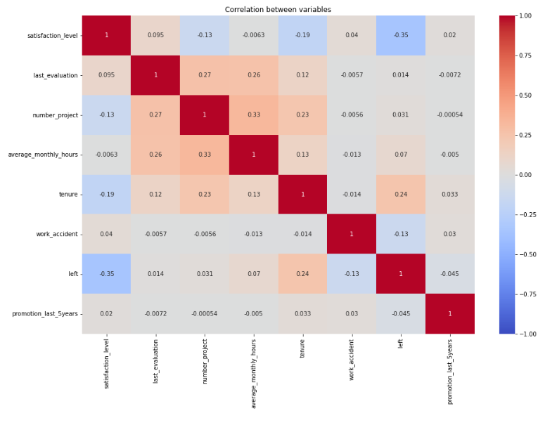
By delving into the distribution of numerical variables and analyzing relationships between them, I made several key observations. The correlation matrix helped me in this regard.
I observed some positive and negative correlations among the variables from the heatmap. The last evaluation, average monthly hours and number of projects are positively correlated with each other. And employee leaving company or not is negatively correlated with satisfaction level. Satisfaction level is also negatively correlated with number of project.
To dig deeper, I plotted more plots with pairwise relationship considering ‘left’ varible.
Relationship 1: satisfaction_level, number_project with left
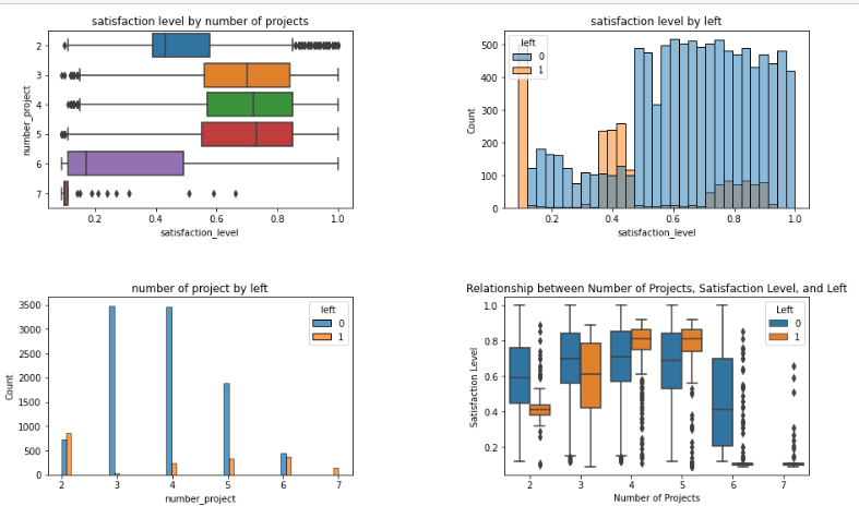
My takeaways from these graphs:
– I noticed a negative correlation between satisfaction level and number of projects, implying that as employees receive more projects, generally 6 or more projects, the satisfaction level then decreases.
– I also observed that employees with lower satisfaction levels are significantly more likely to leave the company, indicating a strong connection between satisfaction and retention.
– Particularly noteworthy is my observation that employees assigned with either 2 projects or 6 or more projects are more prone to leaving compared to those with 3, 4, or 5 projects, suggesting potential dissatisfaction thresholds.
Relationship 2: average_monthly_hours, number project, last_evaluation with left
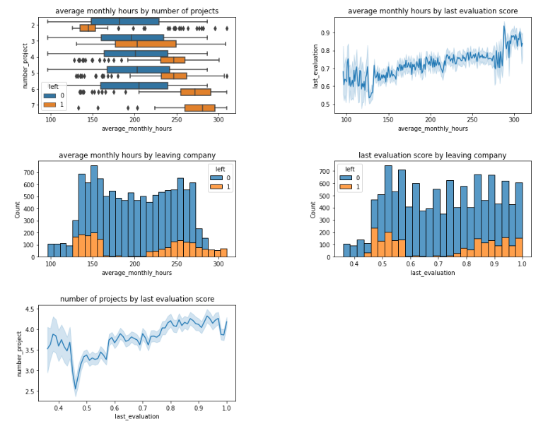
Observations:
- I noticed that employees who left the company typically worked on fewer projects with lower monthly working hours, often around 150 hours per month, and had at most 2 projects. Conversely, employees working more than 250 hours with 6 or more projects showed a higher tendency to leave.
- In the line graphs, I observed that as average monthly hours or number of projects increased, last evaluation scores also tended to increase. However, it’s noteworthy that employees with higher evaluation scores were more likely to leave the company, despite their higher performance ratings.
Relationship 3: Tenure with left
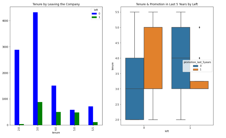
Observations:
- Analyzing the relationship between tenure and leaving the company, I observed a significant trend after employees had worked for approximately 3 years. This suggests that employees are more likely to leave the company after this tenure threshold.
- Further examining the relationship by incorporating promotion_last_5years, I noticed that the majority of promotions occurred during the 3rd to 5th year of tenure. Interestingly, among employees who left the company, the majority did not receive a promotion, indicating a potential correlation between lack of promotion and employee turnover.

Step 3: Build Machine Learning Models
Given the objective of predicting the likelihood of an employee leaving the company, at this modeling phase, I chose to implement 5 machine learning models in total: Logistic Regression, Untuned and Tuned Decision Tree, Random Forest, and XGBoosting. But why 5? It is because I also wanted to bring all things together and apply the skills that I learned from the specialization, and also to compare which model performs better than others. For each of them, I –
- Trained the model with training datasets
- Calculated the predicted values from test data
- Checked assumptions
- Calculated evaluation metrics: accuracy, precision, recall, f1 and AUC
- Checked Confusion Matrix how well the model predicts
- Displayed feature importance by plots.
- Plot other visualizations etc.
The dependent variable (y) was determined to be the “left” variable, indicating whether an employee stayed or left the company. The remaining variables in the dataset, such as satisfaction_level, time_spent_company, and last_evaluation, served as independent variables.
Model no 3: Tuned Decision Tree
After applying logistic regression, I implemented a decision tree which performed far better than the logistic regression. Then, I thought of tuning parameters could give me more better results. So, I implemented another decision tree as my 3rd model. Hyperparameter tuning for a decision tree involves finding the optimal values for parameters that are set before the learning process begins. These parameters control the learning process and the structure of the decision tree. The goal of hyperparameter tuning is to improve the performance of the decision tree model by selecting the best combination of hyperparameters.
The list of hyperparameters I tuned for model:
max_depth: This hyperparameter controls the maximum depth of the decision tree. A deeper tree can capture more complex relationships in the data but may lead to overfitting.
min_samples_leaf:This parameter specifies the minimum number of samples required to be at a leaf node. It controls the minimum size of the leaf nodes and can also help prevent overfitting.
min_samples_split: this parameter specifies the minimum number of samples required to split a node. Increasing this value can help prevent overfitting by requiring more samples for a node to split.

Then, after splitting up train and test data, I instantiated a GridSearch variable based on the tuning above and fitted the training data to the GridSearch.
I found that the optimal parameters were a maximum depth of 6, minimum samples per leaf of 2, and minimum samples for split of 6. The resulting best score of AUC, achieved by the tuned model was 0.9767, indicating very good accuracy on the training data.
I then plotted the decision tree. As the tree was difficult to observe, I exported the tree as text, It gave me nicer combinations from root to till nodes of each combination. This picture only shows part of the tree.
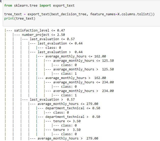
Observation: I recorded all the threshold numbers for all variables when employees leave the company. This is a summary with numbers:
- Employees with satisfaction_level <= 0.47, number_project <= 2.5, last_evaluation > 0.44, and average_monthly_hours > 125.50 are more prone to leave.
- Similar conditions apply when satisfaction_level is <= 0.47, number_project is <= 2.5, last_evaluation is > 0.44, and average_monthly_hours is between 162.00 and 234.00.
- Those with satisfaction_level <= 0.47, number_project <= 2.50, last_evaluation > 0.57, and average_monthly_hours > 279 also exhibit a likelihood of leaving.
- Additionally, employees with satisfaction_level <= 0.11 and number_project > 2.50, or satisfaction_level < 0.11 with number_project > 6.5 show a tendency to leave.
- Further, individuals with satisfaction_level between 0.11 and 0.47 and number_project > 6.5 are prone to leaving as well.
- Employees also leave when satisfaction_level > 0.47, 4.5 < tenure, 1 > last_evaluation > 0.81, average_monthly_hours <= 216
- Lastly, with satisfaction_level > .72, 4.5 < tenure <= 5.25, last_evaluation > 0.81, average_monthly_hours >216, number_project > 3.5, there seems a turnover.
Feature Importance
From the feature importance plot, it is clear that satisfaction_level, last_evaluation, _number_project, average_monthly_hours, and tenure are the most importance features to describe the “left” variable, especially class 1 (left the company).

Decision Tree Results

Evaluation Scores: This model gave the best evaluation scores of all the machine learning models I tried for this project.
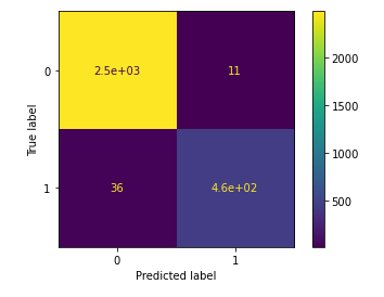
I cross-checked again with this confusion matrix, where it shows the model only has 11 false positives and only 36 false negative values, describing a strong performance.
Comparison of all models
Now, before I share my recommendation with the stakeholders of the project, I would like to share the summary table for all the machine learning models I implemented.
Please consider checking the details of the implemented models from here.
As noticed, there is a fight between my 2nd decision tree and the random forest model. The random forest has better recall and AUC score, but I gave the first place to the decision tree by considering the f1 score. But the point to note here, both models performed better, and insights gathered from both are quite similar.

Step 4: Summarize Results and Provide Recommendations
Recommendations to the Stakeholders
What business recommendations do you propose based on the models built?
The company should prioritize attention towards employees exhibiting low satisfaction levels, receiving lower evaluations, and working more than the average monthly hours. These indicators strongly suggest a higher likelihood of employee turnover, warranting proactive measures to address their concerns and improve retention.
What potential recommendations would you make to your manager/company?
- Set a limit for satisfaction level, continue the survey on a quarterly basis, and counsel with the employee when someone has a lower level.
- Reconsider to change the evaluation score based on the number of hours of work worked, instead assign higher scores of the employee who gives more effort to the project.
- Set a lower & higher threshold for the number of projects assigned to each employee.
- Explore promoting employees working for at least 4 years, or investigate why still they are not.
- Reward employees who work longer hours or just notify them to avoid that, implement a sign-in and out system team-to-team so make employees punctuational and responsible.
- Initiate more cultural and open discussions at both company-wide and team levels to improve the work culture
Do you think your model could be improved Why or why not? How?
- As all variables were considered to all variables, random forest and xgboosting took a lot of time to train the model. Feature engineering could be done after the decision tree results, choosing fewer X variables could save time.
- As the dataset was imbalanced, the logistic regression could not perform well.
- The validation dataset could be defined along with training and testing data to cross-validate to ensure reliable performance.
- To enhance the random forest and XGBoost models, considering a broader range of hyperparameters for tuning can lead to better-performing models.
The following templete I used to showcase the project as an executive summary.
